
Loading...
Loading...
Loading...
Loading...
Loading...
Loading...
Loading...
Loading...
Loading...
Loading...
Loading...
Loading...
Loading...
Loading...
Loading...
Loading...
Loading...
Loading...
Loading...
Loading...
Loading...
Loading...
Loading...
Loading...
Loading...
Loading...
Loading...
Loading...
Loading...
Loading...
Loading...
Loading...
Loading...
Loading...
Loading...
Loading...
Loading...
Loading...
Loading...
Loading...
Loading...
Loading...
Loading...
Loading...
Loading...
Loading...
Loading...
Loading...
Loading...
Loading...
Loading...
Loading...
Loading...
Loading...
Loading...
Loading...
Loading...
Loading...
Loading...
💼 Useful tools in the context of Deep Learning
Visualize the graph of the network
Watch the inputs and outputs of each layer in your CNN
🚀 Download images by class
💁♀️ Download bulk links by one click
👩💻 Google Chrome extension
👩🏫 Concepts of neural network with theoric details
👩🏫 Concepts of neural network with theoric details
A neural network is a type of machine learning which models itself after the human brain. This creates an artificial neural network that via an algorithm allows the computer to learn by incorporating new data.
Neural networks are able to perform what has been termed deep learning. While the basic unit of the brain is the neuron, the essential building block of an artificial neural network is a perceptron which accomplishes simple signal processing, and these are then connected into a large mesh network.
There are many types of neural networks, choosing a type is due to the problem that we are trying to solve, for example
Type
Description
Application
👼 Standard NN
We input some features and estimate the output
Online Advertising, Real Estate
🎨 CNN
We add convolutions for feature extraction
Photo Tagging
🔃 RNN
Suitable for sequence data
Machine Translation, Speech Recognition
🤨 Custom NN / Hybrid
For complex problems
Autonomous Driving
🚧 Structured Data
Such as tables
We have input fields and an output field
🤹♂️ Unstructured Data
Such as images, audio and texts
We need to use feature extraction algorithms to build our model
🥽 Popular Strategies Used In the Context of Deep Learning
Term
Description
🚙 Transfer Learning
Learning form one task and applying knowledge to seperate tasks 🛰🚙
➰ Multi-Task Learning
Starting simultaneously trying to have one NN do several things at same time and then each of these tasks helps all of the other tasks 🚀
🏴 End to End Deep Learning
Breaking the big task into sub smaller tasks with the same NN ✂
🚪 Beginning to solve problems of computer vision with Tensorflow and Keras
🔦 Convolutional Neural Networks Codes
Asmaa Mirkhan's notes (and codes) on deep learning
🕸 My notes about Artificial Neural Networks, Convolutional Neural Networks and Recurrent Neural Networks with theoretical details
🦋 I will share new details as I learn new concepts in this context
Turkish version of this project is
"Your learning algorithm has two main sources of knowledge; one is the data and other is whatever you hand design" 🤔🚀
✨ Help me to improve and to increase the content by opening a pull request
👓 Tell me your suggestions by sending me an or opening an issue
Find me on and feel free to mail me,
🙄 Problems that we can face while training custom object detection
Model is not doing well on test set
Model is doing well on test set but doing bad on real world images
In case that model is not doing well on test set you can try one or more from the followings:
Add dropout to .config file
Replace fixed_shape_resizer with keep_aspect_ratio_resizer, example:
👮♀️ You have to choose these values due to your model
#
Title
0.
1.
2.
3.
4.
5.
6.
7.
8.
9.
#
Title
0.
1.
Term
Description
💫 Convolutoin
Applying some filter on an image so certain features in the image get emphasized
🌀 Pooling
A way of compressing an image
🔷 2*2 max pooling
For every 4 neighbor pixels the biggest one will survive
⭕ Padding
Adding additional border(s) to the image before convolution
👷♀️ Guidelines for Structuring Machine Learning Projects
One of the challenges with building machine learning systems is that there are so many things we could try. Including, for example, so many hyperparameters we could tune. The art of knowing what parameter to tune to get what effect, is called orthogonalisation.
What should we pay attention to while evaluating an ML project? How to optimize it? How to speed up? Since there are a lot of parameters how to know where to fix and which parameter to tune? 🤔🤕
Before answering these questions let's take a look at the whole process 🧐
The model should:
Fit training set well on cost function (Human level performance ❌❌)
⬇
Fit dev set well on cost function
⬇
Fit test set well on cost function
⬇
Perform well in real world ✨
Figuring out what is exactly wrong can help us to choose a suitable solution and then to fix that part without affecting the whole project 👩🔧
Mixed Info On Natural Language Processing
A machine translation model is similar to a language model except it has an encoder network placed before.
It is sometimes referred as a conditional language model.
If you had to translate a book's paragraph from French to English, you would not read the whole paragraph, then close the book and translate 😅
Even during the translation process, you would read/re-read and focus on the parts of the French paragraph corresponding to the parts of the English you are writing down 🤔
The attention mechanism tells a Neural Machine Translation model where it should pay attention to at any step 👩🏫
Converting an audio (x-input) to text (y-output)
By measuring air pressure 🙄
Sequence-to-Sequence model
TODO: Add details
box_predictor {
....
use_dropout: true
dropout_keep_probability: 0.8
....
}Multi class problems
We can learn it by likening it to logistic regression: 😋
Recall that logistic regression produces a decimal between 0 and 1.0. For example, a logistic regression output of 0.8 from an email classifier suggests an 80% chance of an email being spam and a 20% chance of it being not spam. Clearly, the sum of the probabilities of an email being either spam or not spam is 1.0.
Softmax extends this idea into the MULTI-CLASS world. That is, Softmax assigns decimal probabilities to each class in a multi-class problem. Those decimal probabilities must add up to 1.0.
Its other name is Maximum Entropy (MaxEnt) Classifier
We can say that softmax regression generalizes logistic regression
Logistic regression is a special status of softmax where C = 2 🤔
C = number of classes = number of units of the output layer So, is a (C, 1) dimensional vector.
Softmax is implemented through a neural network layer just before the output layer. The Softmax layer must have the same number of nodes as the output layer.
Takes the output of softmax layer and convert it into 1 vs 0 vector (as I called it 🤭) which will be our ŷ
For example:
t = 0.13 ==> ̂y = 0
0.75 1
0.01 0
0.11 0And so on 🐾
Y and ŷ are (C,m) dimensional matrices 👩🔧
Preventing overfitting
Briefly: A technique to prevent overfitting -and reduce variance-
In over-fitting situation, our model tries to learn too well the details and the noise from the training data, which ultimately results in poor performance on the unseen data (test set).
The following graph describes better:
It is a technique which makes slight modifications to the learning algorithm such that the model generalizes better. This in turn improves the model’s performance on the unseen data as well.
The most common type of regularization, given by following formula:
Here, lambda is the regularization parameter. It is the hyperparameter whose value is optimized for better results. L2 regularization is also known as weight decay as it forces the weights to decay towards zero (but not exactly zero)
Another regularization method by eliminating some neurons in a specific ratio randomly
Simply: For each node of probability p, don’t update its input or output weights during backpropagation (Just drop it 😅)
Better visualiztion:
An NN before and after dropout
It is commonly used in computer vision, but its downside is that Cost function J is no longer well defined
The simplest way to reduce overfitting is to increase the size of the training data, it is not always possible since getting more data is too costly, but sometimes we can increase our data based on our data, for example:
Doing transformations on images can maximize our data set
It is a kind of cross-validation strategy where we keep one part of the training set as the validation set. When we see that the performance on the validation set is getting worse, we immediately stop the training on the model. This is known as early stopping.
Long Story Short 😅: Overfitting and Regularization in Neural Networks
Visualization of concepts explained in P1 and P2 to wrap them up 👩🎓
Applying a filter to extract features 🤗
Problem 😰: Images are shrinking 😱
Images Are Too Large, Performance is Down 😔
Filters must have depth that is equal to number of color channels
n filtersDepth of the output will be equal to n
Other Strategies of Deep Learning
In short: We start simultaneously trying to have one NN do several things at same time and then each of these tasks helps all of the other tasks 🚀
In other words: Let's say that we want to build a detector to detect 4 classes of objects, instead of building 4 NN for each class, we can build one NN to detect the four classes 🤔 (The output layer has 4 units)
🤳 Training on a set of tasks that could benefit from having shared lower level features
⛱ Amount of data we have for each task is quite similar (sometimes) ⛱
🤗 Can train a big enough NN to do well on all the tasks (instead of building a separate network fır each task)
👓 Multi task learning is used much less than transfer learning
Briefly, there have been some data processing systems or learning systems that requires multiple stages of processing,
End to end learning can take all these multiple stages and replace it with just a single NN
👩🔧 Long Story Short: breaking the big task into sub smaller tasks with the same NN
🦸♀️ Shows the power of the data
✨ Less hand designing of components needed
💔 May need large amount of data
🔎 Excludes potentially useful hand designed components
Key question: do you have sufficient data to learn a function of the complexity needed to map x to y?
👀 Visual materials to give lots of information in short time
Materials will be divided into different files (or categories) as they increase 👮
We did element wise product then we get the sum of the result matrix; so:
And so on for other elements 🙃
An application of convolution operation
Result: horizontal lines pop out
Result: vertical lines pop out
There are a lot of ways we can put number inside elements of the filter.
For example Sobel filter is like:
Scharr filter is like:
Prewitt filter is like:
So the point here is to pay attention to the middle row
And Roberts filter is like:
We can tune these numbers by ML approach; we can say that the filter is a group of weights that:
By that we can get -learned- horizontal, vertical, angled, or any edge type automatically rather than getting them by hand.
If we have an n*n image and we convolve it by f*f filter the the output image will be n-f+1*n-f+1
🌀 If we apply many filters then our image shrinks.
🤨 Pixels at corners aren't being touched enough, so we are throwing away a lot of information from the edges of the image .
We can the image 💪
During each iteration of training a neural network, all weights receive an update proportional to the partial derivative of the error function with respect to the current weight. If the gradient is very small then the weights will not be change effectively and it may completely stop the neural network from further training 🙄😪. The phenomenon is called vanishing gradients 🙁
Simply 😅: we can say that the data is disappearing through the layers of the deep neural network due to very slow gradient descent
The core idea of ResNet is introducing a so-called identity shortcut connection that skips one or more layers, like the following
Easy for one of the blocks to learn an identity function
Can go deeper without hurting the performance
In the Plain NNs, because of the vanishing and exploding gradients problems the performance of the network suffers as it goes deeper.
We can reduce the size of inputs by applying pooling and various convolution, these filteres can reduce the height and the width of the input image, what about color channels 🌈, in other words; what about the depth?
We know that the depth of the output of a CNN is equal to the number of filters that we applied on the input;
In the example above, we applied 2 filters, so the output depth is 2
How can we use this info to improve our CNNs? 🙄
Let's say that we have a 28x28x192 dimensional input, if we apply 32 filters at 1x1x192 dimension and padding our output will become 28x28x32 ✨
Make your training procedure more effective
While looking to precesion P and recall R (for example) we may be not able to choose the best model correctly
So we have to create a new evaluation metric that makes a relation between P and R
Now we can choose the best model due to our new metric 🐣
For example: (as a popular associated metric) F1 Score is:
To summarize: we can construct our own metrics due to our models and values to be able to get the best choice 👩🏫
For better evaluation we have to classify our metrics as the following:
Technically, If we have N metrics we have to try to optimize 1 metric and to satisfice N-1 metrics 🙄
🙌 Clarification: we tune satisficing metrics due to a threshold that we determine
It is recommended to choose the dev and test sets from the same distribution, so we have to shuffle the data randomly and then split it.
As a result, both test and dev sets have data from all categories ✨
We have to choose a dev set and test set - from same distribution - to reflect data we expect to get in te future and consider important to do well on
If we have a small dataset (m < 10,000)
60% training, 20% dev, 20% test will be good
If we have a huge dataset (1M for example)
99% trainig, %1 dev, 1% test will be acceptable
And so on, considering these two statuses we can choose the correct ratio 👮
Guideline: if doing well on metric + dev/test set and doesn't correspond to doing well in the real world application, we have to change our metric and/or dev/test set 🏳
🕵️♀️ Popular Object Detection Techniques
R-CNN (Regional Based Convolutional Neural Networks)
Fast R-CNN (Regional Based Convolutional Neural Networks)
Faster R-CNN (Regional Based Convolutional Neural Networks)
RFCN (Region Based Fully Connected Convolutional Neural Networks)
YOLO (You Only Look Once)
YOLO V1
YOLO V2
YOLO V3
SSD (Single Shot Detection)
General Concepts of Sequence Models
In the context of text processing (e.g: Natural Language Processing NLP)
A way to represent words so we can treat with them easily
Let's say that we have a dictionary that consists of 10 words (🤭) and the words of the dictionary are:
Car, Pen, Girl, Berry, Apple, Likes, The, And, Boy, Book.
Our $$X^{(i)}$$ is: The Girl Likes Apple And Berry
So we can represent this sequence like the following 👀
By representing sequences in this way we can feed out data to neural networks ✨
If our dictionary consists of 10,000 words so each vector will be 10,000 dimensional 🤕
This representation can not capture semantic features 💔
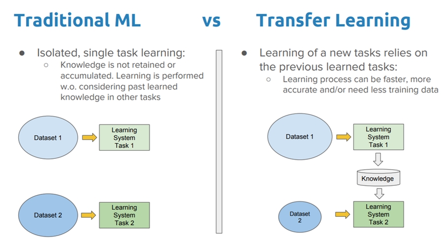
Applying a knowledge to separate tasks
In short: Learning from one task and applying knowledge to separate tasks 🛰🚙
🕵️♀️ Transfer learning is a machine learning technique where a model trained on one task is re-purposed on a second related task.
🌟 In addition, it is an optimization method that allows rapid progress or improved performance when modeling the second task.
🤸♀️ Transfer learning only works in deep learning if the model features learned from the first task are general.
Long story short: Rather than training a neural network from scratch we can instead download an open-source model that someone else has already trained on a huge dataset maybe for weeks and use these parameters as a starting point to train our model just a little bit more with the smaller dataset that we have ✨
Layers in a neural network can sometimes end up having similar weights and possible impact each other leading to over-fitting. With a big complex model it's a risk. So if you can imagine the dense layers can look a little bit like this.
We can drop out some neurons that has similar weights with neighbors, so that overfitting is being removed.
🤸♀️ An NN before and after dropout
✨ Accuracy before and after dropout
It is practical when we have a lot of data for problem that we are transferring from and usually relatively less data for the problem we are transferring to 🕵️
More accurately:
For task A to task B, it is sensible to do transfer learning from A to B when:
🚩 Task A and task B have the same output x
⭐ We have a lot more data for task A than task B
🔎 Low level features from task A could be helpful for learning task B
Metric Type
Description
✨ Optimizing Metric
A metric that has to be in its best value
🤗 Satisficing Metric
A metric that just has to be good enough
Symbol
Description
$$X^{}$$
The tth word in the input sequence
$$Y^{}$$
The tth word in the output sequence
$$X^{(i)}$$
The tth word in the ith input sequence
$$Y^{(i)}$$
The tth word in the ith output sequence
$$T^{(i)}_x$$
The length of the ith input sequence
$$T^{(i)}_y$$
The length of the ith output sequence
Car -0) ⌈ 0 ⌉ ⌈ 0 ⌉ ⌈ 0 ⌉ ⌈ 0 ⌉ ⌈ 0 ⌉ ⌈ 0 ⌉
Pen -1) | 0 | | 0 | | 0 | | 0 | | 0 | | 0 |
Girl -2) | 0 | | 1 | | 0 | | 0 | | 0 | | 0 |
Berry -3) | 0 | | 0 | | 0 | | 0 | | 0 | | 1 |
Apple -4) | 0 | | 0 | | 0 | | 1 | | 0 | | 0 |
Likes -5) | 0 | | 0 | | 1 | | 0 | | 0 | | 0 |
The -6) | 1 | | 0 | | 0 | | 0 | | 0 | | 0 |
And -7) | 0 | | 0 | | 0 | | 0 | | 1 | | 0 |
Boy -8) | 0 | | 0 | | 0 | | 0 | | 0 | | 0 |
Book -9) ⌊ 0 ⌋ ⌊ 0 ⌋ ⌊ 0 ⌋ ⌊ 0 ⌋ ⌊ 0 ⌋ ⌊ 0 ⌋🚪 Beginning to solve problems of computer vision with Tensorflow and Keras
The MNIST database: (Modified National Institute of Standards and Technology database)
🔎 Fashion-MNIST is consisting of a training set of 60,000 examples and a test set of 10,000 examples
🎨 Types:
🔢 MNIST: for handwritten digits
👗 Fashion-MNIST: for fashion
📃 Properties:
🌚 Grayscale
28x28 px
10 different categories
Term
Description
➰ Sequential
That defines a SEQUENCE of layers in the neural network
⛓ Flatten
Flatten just takes that square and turns it into a 1 dimensional set (used for input layer)
🔷 Dense
Adds a layer of neurons
💥 Activation Function
A formula that introduces non-linear properties to our Network
✨ Relu
An activation function by the rule: If X>0 return X, else return 0
🎨 Softmax
An activation function that takes a set of values, and effectively picks the biggest one
The main purpose of activation function is to convert a input signal of a node in a NN to an output signal. That output signal now is used as a input in the next layer in the stack 💥
Values in MNIST are between 0-255 but neural networks work better with normalized data, so we can divide every value by 255 so the values are between 0,1.
There are multiple criterias to stop training process, we can specify number of epochs or a threshold or both
Epochs: number of iterations
Threshold: a threshold for accuracy or loss after each iteration
Threshold with maximum number of epochs
We can check the accuracy at the end of each epoch by Callbacks 💥
Notes on Implementing CNNs In The Browser
To implement our CNN based works in the Browser we need to use Tensorflow.JS 🚀
🚙 Import Tensorflow.js
👷♀️ Create models
👩🏫 Train
👩⚖️ Do inference
We can import Tensorflow.js in the way below
<script
src="https://cdn.jsdelivr.net/npm/@tensorflow/tfjs@latest">
</script>😎 Same as we did in Python:
🐣 Decalre a Sequential object
👩🔧 Add layers
🚀 Compile the model
👩🎓 Train (fit)
🐥 Use the model to predict
// create sequential
const model = tf.sequential();
// add layer(s)
model.add(tf.layers.dense({units: 1, inputShape: [1]}));
// set compiling parameters and compile the model
model.compile({loss:'meanSquaredError',
optimizer:'sgd'});
// get summary of the mdoel
model.summary();
// create sample data set
const xs = tf.tensor2d([-1.0, 0.0, 1.0, 2.0, 3.0, 4.0], [6, 1]);
const ys = tf.tensor2d([-3.0, -1.0, 2.0, 3.0, 5.0, 7.0], [6, 1]);
// train
doTraining(model).then(() => {
// after training
predict = model.predict(tf.tensor2d([10], [1,1]));
predict.print();
});
([-1.0, 0.0, 1.0, 2.0, 3.0, 4.0], [6, 1])
[-1.0, 0.0, 1.0, 2.0, 3.0, 4.0]: Data set values
[6, 1]: Shape of input
👁🗨 Attention
🐢 Training is a long process so that we have to do it in an asynchronous function
async function doTraining(model){
const history =
await model.fit(xs, ys,
{ epochs: 500,
callbacks:{
onEpochEnd: async(epoch, logs) =>{
console.log("Epoch:"
+ epoch
+ " Loss:"
+ logs.loss);
}
}
});
}image_resizer {
fixed_shape_resizer {
height: 640
width: 640
}
}keep_aspect_ratio_resizer {
min_dimension: 640
max_dimension: 640
pad_to_max_dimension: true
}Term
Description
Convolution
Applying some filter on an image so certain features in the image get emphasized
3*1 + 1*0 + 1*(-1)
+
1*1 + 0*0 + 7*(-1)
+
2*1 + 3*0 + 5*(-1)
=
-71 0 -1
2 0 -2
1 0 -13 0 -3
10 0 -10
3 0 -3-1 0 1
-1 0 1
-1 0 11 0
0 -1w1 w2 w3
w4 w5 w6
w7 w8 w9Approach
Description
Residual Networks
An approach to avoid vanishing gradient issue in deep NNs
One By One Convolution
Applying filters on color channels
Term
Description
Classification
Specifying the label (class) of an object in input image
Classification and Localization
Specifying the label and coordinates of an object in input image
Object Detection
Specifying labels and coordinates of multiple objects in input image
Classification
Clf. and Localization
Detection
#of objects
1
1
multiple
Input
image
image
image
Output
label
label + coordinates
label(s) + coordinates
👩💻 Intro to Neural Networks Coding
Like every first app we should start with something super simple that gives us an idea about the whole methodology.
Keras is a high-level neural networks API, written in Python and capable of running on top of TensorFlow, CNTK, or Theano.
Term
Description
Dense
A layer of neurons in a neural network
Loss Function
A mathematical way of measuring how wrong your predictions are
Optimizer
An algorithm to find parameter values which correspond to minimum value of loss function
It contains one layer with one neuron.
# initialize the model
model = Sequential()
# add a layer with one unit and set the dimension of input
model.add(Dense(units=1, input_shape=[1]))
# set functional properties and compile the model
model.compile(optimizer='sgd', loss='mean_squared_error'After building out neural network we can feed it with our sample data 😋
xs = np.array([-1.0, 0.0, 1.0, 2.0, 3.0, 4.0], dtype=float)
ys = np.array([-3.0, -1.0, 1.0, 3.0, 5.0, 7.0], dtype=float)Then we have to start training process 🚀
model.fit(xs, ys, epochs=500)Every thing is done 😎 ! Now we can test our neural network with new data 🎉
print(model.predict([10.0]))Given a dataset like:
We want:
Concept
Description
m
Number of examples in dataset
ith example in the dataset
ŷ
Predicted output
Loss Function 𝓛(ŷ, y)
A function to compute the error for a single training example
Cost Function 𝙹(w, b)
The average of the loss functions of the entire training set
Convex Function
A function that has one local value
Non-Convex Function
A function that has lots of different local values
Gradient Descent
An iterative optimization method that we use to converge to the global optimum of Cost Function
In other words: The
Cost Functionmeasures how well our parameterswandbare doing on the training set, so the bestwandbare the values that minimize𝙹(w, b)as possible
General Formula:
α(alpha) is the Learning Rate
It is a positive scalar determining the size of the step of each iteration of gradient descent due to the corresponded estimated error each time the model weights are updated, so, it controls how quickly or slowly a neural network model learns a problem.
The main purpose of Activation Functions is to convert an input signal of a node in an ANN to an output signal by applying a transformation. That output signal now is used as a input in the next layer in the stack.
Formula:
Graph:
It can be used in regression problem in the output layer
Formula:
Graph:
Almost always strictly superior than sigmoid function
Formula:
Shifted version of the Sigmoid function 🤔
Graph:
Activation functions can be different for different layers, for example, we may use tanh for a hidden layer and sigmoid for the output layer
If z is very large or very small then the derivative (or the slope) of these function becomes very small (ends up being close to 0), and so this can slow down gradient descent 🐢
Another and very popular choice
Formula:
Graph:
So the derivative is 1 when z is positive and 0 when z is negative
Disadvantage: derivative=0 when z is negative 😐
Formula:
Graph:
Or: 😛
A lot of the space of z the derivative of the activation function is very different from 0
NN will learn much faster than when using tanh or sigmoid
Well, if we use linear function then the NN is just outputting a linear function of the input, so no matter how many layers out NN has 🙄, all it is doing is just computing a linear function 😕
❗ Remember that the composition of two linear functions is itself a linear function
If the output is 0 or 1 (binary classification) ➡ sigmoid is good for output layer
For all other units ➡ Relu ✨
We can say that relu is the default choice for activation function
Note:
If you are not sure which one of these functions work best 😵, try them all 🤕 and evaluate on different validation set and see which one works better and go with that 🤓😇
Single Shot Detectors and You Only Look Once
💥 The approach involves a single neural network trained end to end
It takes an image as input and predicts bounding boxes and class labels for each bounding box directly.
😕 The technique offers lower predictive accuracy (e.g. more localization errors) Compared with region based models
➗ YOLO divides the input image into an S×S grid. Each grid cell predicts only one object
👷♀️ Long Story Short: The system divides the input image into an S × S grid. If the center of an object falls into a grid cell, that grid cell is responsible for detecting that object.
🚀 Speed
🤸♀️ Feasible for real time applications
😕 Poor performance on small-sized objects
It tends to give imprecise object locations.
TODO: Compare versions of YOLO
💥 Predicts objects in images using a single deep neural network.
🤓 The network generates scores for the presence of each object category using small convolutional filters applied to feature maps.
✌ This approach uses a feed-forward CNN that produces a collection of bounding boxes and scores for the presence of certain objects.
❗ In this model, each feature map cell is linked to a set of default bounding boxes
🖼️ After going through a certain of convolutions for feature extraction, we obtain a feature layer of size m×n (number of locations) with p channels, such as 8×8 or 4×4 above.
And a 3×3 conv is applied on this m×n×p feature layer.
📍 For each location, we got k bounding boxes. These k bounding boxes have different sizes and aspect ratios.
The concept is, maybe a vertical rectangle is more fit for human, and a horizontal rectangle is more fit for car.
💫 For each of the bounding boxes, we will compute c class scores and 4 offsets relative to the original default bounding box shape.
The SSD object detection algorithm is composed of 2 parts:
Extract feature maps
Apply convolution filters to detect objects.
Better accuracy compared to YOLO
Better speed compared to Region based algorithms
Adding an additional one border or more to the image so the image is n+2 x n+2 and after convolution we end up with n x n image which is the original size of the image
p = number of added borders
For convention: it is filled by 0
For better understanding let's say that we have two concepts:
It means no padding so:
n x n * f x f ➡ n-f+1 x n-f+1
Pad so that output size is the same as the input size.
So we want that 🧐:
n+2p-f+1 = n
Hence:
p = (f-1)/2
For convention f is chosen to be odd 👩🚀
Another approach of convolutions, we calculate the output by applying filter on regions by some value s.
For an n x n image and f x f filter, with p padding and stride s; the output image size can be calculated by the following formula
To apply convolution operation on an RGB image; for example on 10x10 px RGB image, technically the image's dimension is 10x10x3 so we can apply for example a 3x3x3 filter or fxfx3 🤳
Filters can be applied on a special color channel 🎨
👩🏫 Usually when people report number of layers in an NN they just report the number of layers that have weights and params
Convention:
CONV1+POOL1=LAYER1
Better performance since they decrease the parameters that will be tuned 💫
Implementation guidelines and error anlysis
Well, in this stage we have a criteria, is your model doing worse than humans (Because humans are quite good at a lot of tasks 👩🎓)? If yes, you can:
👩🏫 Get labeled data from humans
👀 Gain insight from manual error analysis; (Why did a person get this right? 🙄)
🔎 Better analysis of bias / variance 🔍
🤔 Note: knowing how well humans can do on a task can help us to understand better how much we should try to reduce bias and variance
Processes are less clear 😥
Suitable techniques will be added here
Let's assume that we have these two situations:
Even though training and dev errors are same we will apply different tactics for better performance
In Case1, We have High Bias so we have to focus on bias reduction techniques 🤔, in other words we have to reduce the difference between training and human errors the avoidable error
Better algorithm, better NN structure, ......
In Case2, We have High Variance so we have to focus on variance reduction techniques 🙄, in other words we have to reduce the difference between training and dev errors
Adding regularization, getting more data, ......
We call this procedure of analysis Error analysis 🕵️
In computer vision issues,
human-level-error ≈ bayes-errorbecause humans are good in vision tasks
Online advertising
Product recommendations
Logistics
Loan approvals
.....
When we have a new project it is recommended to produce an initial model and then iterate over it until you get the best model, this is more practical than spending time building model theoretical and thinking about the best hyperparameter -which is almost impossible 🙄-
So, just don't overthink! (In both ML problems and life problems 🤗🙆)
LeNet-5 is a very simple network - By modern standards -. It only has 7 layers;
among which there are 3 convolutional layers (C1, C3 and C5)
2 sub-sampling (pooling) layers (S2 and S4)
1 fully connected layer (F6)
Output layer
Too similar to LeNet-5
It has more filters per layer
It uses ReLU instead of tanh
SGD with momentum
Uses dropout instead of regularaization
It is painfully slow to train (It has 138 million parameters 🙄)
⛓ Basics of Sequence Models
Sequences are data structures where each example could be seen as a series of data points, for example 🧐:
Since we have labeled data X and Y so all of these tasks are addressed as Supervised Learning 👩🏫
Even in Sequence-to-Sequence tasks lengths of input and output can be different ❗
Machine learning algorithms typically require the text input to be represented as a fixed-length vector 🙄
Thus, to model sequences, we need a specific learning framework able to:
✔ Deal with variable-length sequences
✔ Maintain sequence order
✔ Keep track of long-term dependencies rather than cutting input data too short
✔ Share parameters across the sequence (so not re-learn things across the sequence)
Task
Input X
Output Y
Type
💬 Speech Recognition
Wave sequence
Text sequence
Sequence-to-Sequence
🎶 Music Generation
Nothing / Integer
Wave Sequence
One-to_Sequence
💌 Sentiment Classification
Text Sequence
Integer Rating (1➡5)
Sequence-to-One
🔠 Machine Translation
Text Sequence
Text Sequence
Sequence-to-Sequence
📹 Video Activity Recognition
Video Frames
Label
Sequence-to-One
Brief Introduction to Tensorflow
Create Tensors (variables) that are not yet executed/evaluated.
Write operations between those Tensors.
Initialize your Tensors.
Create a Session.
Run the Session. This will run the operations you'd written above.
To summarize, remember to initialize your variables, create a session and run the operations inside the session. 👩🏫
To calculate the following formula:
# Creating tensors and writing operations between them
y_hat = tf.constant(36, name='y_hat')
y = tf.constant(39, name='y')
loss = tf.Variable((y - y_hat)**2, name='loss')
# Initializing tensors
init = tf.global_variables_initializer()
# Creating session
with tf.Session() as session:
# Running the operations
session.run(init)
# printing results
print(session.run(loss))When we created a variable for the loss, we simply defined the loss as a function of other quantities, but did not evaluate its value. To evaluate it, we had to use the initializer.
For the following code:
a = tf.constant(2)
b = tf.constant(10)
c = tf.multiply(a,b)
print(c)🤸♀️ The output is
Tensor("Mul:0", shape=(), dtype=int32)As expected, we will not see 20 🤓! We got a tensor saying that the result is a tensor that does not have the shape attribute, and is of type "int32". All we did was put in the 'computation graph', but we have not run this computation yet.
A placeholder is an object whose value you can specify only later. To specify values for a placeholder, we can pass in values by using a feed dictionary.
Below, a placeholder has been created for x. This allows us to pass in a number later when we run the session.
x = tf.placeholder(tf.int64, name = 'x')
print(sess.run(2 * x, feed_dict = {x: 3}))
sess.close()Computing sigmoid function with TF
def sigmoid(z):
"""
Computes the sigmoid of z
Arguments:
z -- input value, scalar or vector
Returns:
results -- the sigmoid of z
"""
# Creating a placeholder for x. Naming it 'x'.
x = tf.placeholder(tf.float32, name = 'x')
# computing sigmoid(x)
sigmoid = tf.sigmoid(x)
# Creating a session, and running it.
with tf.Session() as sess:
# Running session and call the output "result"
result = sess.run(sigmoid, feed_dict = {x: z})
return resultComputing cost function with TF
def cost(logits, labels):
"""
Computes the cost using the sigmoid cross entropy
Arguments:
logits -- vector containing z, output of the last linear unit (before the final sigmoid activation)
labels -- vector of labels y (1 or 0)
Returns:
cost -- runs the session of the cost function
"""
# Creating the placeholders for "logits" (z) and "labels" (y)
z = tf.placeholder(tf.float32, name = 'z')
y = tf.placeholder(tf.float32, name = 'y')
# Using the loss function
cost = tf.nn.sigmoid_cross_entropy_with_logits(logits = z, labels = y)
# Creating a session
sess = tf.Session()
# Running the session
cost = sess.run(cost, feed_dict = {z: logits, y: labels})
# Closing the session
sess.close()
return cost🔦 Convolutional Neural Networks Codes
This section will be filled by codes and notes gradually
🌐 Tensorflow.js based hand written digit recognizer
Rock Paper Scissors is an available dataset containing 2,892 images of diverse hands in Rock/Paper/Scissors poses.
Rock Paper Scissors contains images from a variety of different hands, from different races, ages and genders, posed into Rock / Paper or Scissors and labelled as such.
🔎 All of this data is posed against a white background. Each image is 300×300 pixels in 24-bit color
We can get info about our CNN by
model.summary()And the output will be like:
Layer (type) Output Shape Param #
=================================================================
conv2d_18 (Conv2D) (None, 26, 26, 64) 640
_________________________________________________________________
max_pooling2d_18 (MaxPooling (None, 13, 13, 64) 0
_________________________________________________________________
conv2d_19 (Conv2D) (None, 11, 11, 64) 36928
_________________________________________________________________
max_pooling2d_19 (MaxPooling (None, 5, 5, 64) 0
_________________________________________________________________
flatten_9 (Flatten) (None, 1600) 0
_________________________________________________________________
dense_14 (Dense) (None, 128) 204928
_________________________________________________________________
dense_15 (Dense) (None, 10) 1290
=================================================================👩💻 For code in the notebook:
Here 🐾
🔎 The original dimensions of the images were 28x28 px
1️⃣ 1st layer: The filter can not be applied on the pixels on the edges
The output of first layer has 26x26 px
2️⃣ 2nd layer: After applying 2x2 max pooling the dimensions will be divided by 2
The output of this layer has 13x13 px
3️⃣ 3rd layer: The filter can not be applied on the pixels on the edges
The output of this layer has 11x11 px
4️⃣ 4th layer: After applying 2x2 max pooling the dimensions will be divided by 2
The output of this layer has 5x5 px
5️⃣ 5th layer: The output of the previous layer will be flattened
This layer has 5x5x64=1600 units
6️⃣ 6th layer: We set it to contain 128 units
7️⃣ 7th layer: Since we have 10 categories it consists of 10 units
😵 😵
The visualization of the output of each layer is available here 🔎
Handling texts using Python's built-in functions
text = "Beauty always reserved in details, don't let the big picture steal your attention!"
len(text)
# 82text = "Beauty always reserved in details, don't let the big picture steal your attention!"
words = text.split(' ')
len(words)
# 13text = "Beauty always reserved in details, don't let the big picture steal your attention!"
words = text.split(' ')
moreThan4 = [w for w in words if len(w) > 4]
# ['Beauty', 'always', 'reserved', 'details,', "don't", 'picture', 'steal', 'attention!']text = "Beauty Always reserved in details, Don't let the big picture steal your attention!"
words = text.split(' ')
capitalized = [w for w in words if w.istitle()]
# ['Beauty', 'Always']
# "Don't" is not found 🙄or specific start .startswith()
text = "You can hide whatever you want to hide but your eyes will always expose you, eyes never lie."
words = text.split(' ')
endsWithEr = [w for w in words if w.endswith('er')]
# ['whatever', 'never']"ESMA".isupper() # True
"Esma".isupper() # False
"esma".isupper() # False
"esma".islower() # True
"ESMA".islower() # False
"Esma".islower() # False'm' in 'esma' # True
'es' in 'esma' # True
'ed' in 'esma' # Falsetext = "To be or not to be"
words = text.split(' ')
unique = set(words)
# {'be', 'To', 'not', 'or', 'to'}text = "To be or not to be"
words = text.split(' ')
unique = set(w.lower() for w in words)
# {'not', 'or', 'be', 'to'}'17'.isdigit() # True
'17.7'.isdigit() # False'esma'.isalpha() # True
'esma17'.isalpha() # False'17esma'.isalnum() # True
'17esma;'.isalnum() # False"Esma".lower() # esma
"Esma".upper() # ESMA
"EsmA".title() # Esmatext = "Beauty,Always,reserved,in,details,Don't,let,the,big,picture,steal,your,attention!"
words = text.split(',')
# ['Beauty', 'Always', 'reserved', 'in', 'details', "Don't", 'let', 'the', 'big', 'picture', 'steal', 'your', 'attention!']text = "Beauty,Always,reserved,in,details,Don't,let,the,big,picture,steal,your,attention!"
words = text.split(',')
joined = " ".join(words)
# Beauty Always reserved in details Don't let the big picture steal your attention!🕵️♀️ Popular Object Detection Techniques
Function
Description
Linear Activation Function
Inefficient, used in regression
Sigmoid Function
Good for output layer in binary classification problems
Tanh Function
Better than sigmoid
Relu Function ✨
Default choice for hidden layers
Leaky Relu Function
Little bit better than Relu, Relu is more popular
Term
Description
🔷 Padding
Adding additional border(s) to the image before convolution
🌠 Strided Convolution
Convolving by s steps
🏐 Convolutions Over Volume
Applying convs on n-dimensional input (such as an RGB image)
Layer
Description
💫 Convolution CONV
Filters to extract features
🌀 Pooling POOL
A technique to reduce size of representation and to speed up the computations
⭕ Fully Connected FC
Standard single neural network layer (one dimensional)
Term
Description
👩🎓 Bayes Error
The lowest possible error rate for any classifier (The optimal error 🤔)
👩🏫 Human Level Error
The error rate that can be obtained by a human
👮♀️ Avoidable Bias
The difference between Bayes error and human level error
Case1
Case2
Human Error
1%
7.5%
Training Error
8%
8%
Dev Error
10%
10%
Network
First Usage
LeNet-5
Hand written digit classification
AlexNet
ImageNet Dataset
VGG-16
ImageNet Dataset
It is a part of data preparation
If we have a feature that is all positive or all negative, this will make learning harder for the nodes in the layer that follows. They will have to zigzag like the ones following a sigmoid activation function.
If we transform our data so it has a mean close to zero, we will thereby make sure that there are both positive values and negative ones.
Formula:
Benifit: It makes cost function J easier and faster to optimize 😋
Number of layers, number of hidden units, learning rates, activation functions...
It is too difficult to choose them all true at the first time so it is an iterative process
Idea ➡ Code ➡ Experiment ➡ Idea 🔁
So the point here is how to go efficiently around this cycle 🤔
For good evaluation it is good to split dataset like the following:
Part
Description
Training Set
Used to fit the model
Development (Validation) Set
Used to provide an unbiased evaluation while tuning model hyperparameters
Test Set
Used to provide an unbiased evaluation of a final model
The actual dataset that we use to train the model (weights and biases in the case of Neural Network).
The model sees and learns from this data 👶
The sample of data used to provide an unbiased evaluation of a model fit on the training dataset while tuning model hyperparameters. The evaluation becomes more biased as skill on the validation dataset is incorporated into the model configuration.
The model sees this data, but never learns from this 👨🚀
The sample of data used to provide an unbiased evaluation of a final model fit on the training dataset. It provides the gold standard used to evaluate the model 🌟.
Implementation Note: Test set should contain carefully sampled data that spans the various classes that the model would face, when used in the real world 🚩🚩🚩❗❗❗
It is only used once a model is completely trained 👨🎓
Bias is how far are the predicted values from the actual values. If the average predicted values are far off from the actual values then the bias is high.
Having high-bias implies that the model is too simple and does not capture the complexity of data thus underfitting the data 🤕
Variance is the variability of model prediction for a given data point or a value which tells us spread of our data.
Model with high variance fails to generalize on the data which it hasn’t seen before.
Having high-variance implies that algorithm models random noise present in the training data and it overfits the data 🤓
If we aren't able to get wanted performance we should ask these questions to improve our model:
We check the performance of the following solutions on dev set
Do we have high bias? If yes, it is a trainig problem, we may:
Try bigger network
Train longer
Try better optimization algorithm
Try another NN architecture
We can say that it is a structural problem 🤔
Do we have high variance? If yes, it is a dev set performance problem, we may:
Get more data
Do regularization
L2, dropout, data augmentation
We can say that maybe it is data or algorithmic problem 🤔
No high variance and no high bias?
TADAAA it is done 🤗🎉🎊
Vanishing Gradients with recurrent neural networks
An RNN that process a sequence data with the size of 10,000 time steps, has 10,000 deep layers which is very hard to optimize 🙄
Same in Deep Neural Networks, deeper networks are getting into the vanishing gradient problem.
That also happens with RNNs with a long sequence size 🐛
GRU Gated Recurrent Unit
LSTM Long Short-Term Memory
GRUs are improved version of standard recurrent neural network ✨, GRU uses update gate and reset gate .
Basically, these are two vectors which decide what information should be passed to the output.
The special thing about them is that they can be trained to keep information from long ago
Without washing it through time or removing information which is relevant to the prediction.
Gate
Description
🔁 Update Gate
Helps the model to determine how much of the past information (from previous time steps) needs to be passed along to the future
0️⃣ Reset Gate
Helps the model to decide how much of the past information to forget
Given this gate the issue of the vanishing gradient is eliminated since the model on its own learn how much of the past information to pass to the future.
In short: How much past should matter now? 🙄
This gate has the opposite functionality in comparison with the update gate since it is used by the model to decide how much of the past information to forget.
In short: Drop previous information? 🙄
Memory content which will use the reset gate to store the relevant information from the past.
A vector which holds information for the current unit and it will pass it further down to the network.
A solution to eliminate the vanishing gradient problem
The model is not washing out the new input every single time but keeps the relevant information and passes it down to the next time steps of the network.
Let's assume we are reading words in a piece of text, and want use an LSTM to keep track of grammatical structures, such as whether the subject is singular or plural.
If the subject changes from a singular word to a plural word, we need to find a way to get rid of our previously stored memory value of the singular/plural state.
In an LSTM, the forget gate let us do this:
$$\Gamma ^{}_f = \sigma(W_f[a^{}, x^{}]+b_f)$$
Here, $W_f$ are weights that govern the forget gate's behavior. We concatenate $$[a^{}, x^{}]$$ and multiply by $$W_f$$. The equation above results in a vector $$\Gamma_f^{}$$ with values between 0 and 1.
This forget gate vector will be multiplied element-wise by the previous cell state $$c^{}$$.
So if one of the values of $$\Gamma_f^{}$$ is 0 (or close to 0) then it means that the LSTM should remove that piece of information (e.g. the singular subject) in the corresponding component of $$c^{}$$ .
If one of the values is 1, then it will keep the information.
Once we forget that the subject being discussed is singular, we need to find a way to update it to reflect that the new subject is now plural. Here is the formula for the update gate:
$$\Gamma ^{}_u = \sigma(W_u[a^{}, x^{}]+b_u)$$
Similar to the forget gate, here $$\Gamma_u^{}$$ is again a vector of values between 0 and 1. This will be multiplied element-wise with $$\tilde{c}^{}$$, in order to compute $$c^{⟨t⟩}$$.
To update the new subject we need to create a new vector of numbers that we can add to our previous cell state. The equation we use is:
$$\tilde{c}^{}=tanh(W_c[a^{}, x^{}]+b_c)$$
Finally, the new cell state is:
$$c^{}=\Gamma _f^{}c^{} + \Gamma _u^{}\tilde{c}^{}$$
To decide which outputs we will use, we will use the following two formulas:
$$\Gamma _o^{}=\sigma(W_o[a^{}, x^{}]+b_o)$$
$$a^{} = \Gamma _o^{}*tanh(c^{})$$
Where in first equation we decide what to output using a sigmoid function and in second equation we multiply that by the tanh of the previous state.
GRU is newer than LSTM, LSTM is more powerful but GRU is easier to implement 🚧
Approaches of word representation
This document may contain incorrect info 🙄‼ Please open a pull request to fix when you find a one 🌟
One Hot Encoding
Featurized Representation (Word Embedding)
Word2Vec
Skip Gram Model
GloVe (Global Vectors for Word Representation)
A way to represent words so we can treat with them easily
Let's say that we have a dictionary that consists of 10 words (🤭) and the words of the dictionary are:
Car, Pen, Girl, Berry, Apple, Likes, The, And, Boy, Book.
Our $$X^{(i)}$$ is: The Girl Likes Apple And Berry
So we can represent this sequence like the following 👀
Car -0) ⌈ 0 ⌉ ⌈ 0 ⌉ ⌈ 0 ⌉ ⌈ 0 ⌉ ⌈ 0 ⌉ ⌈ 0 ⌉
Pen -1) | 0 | | 0 | | 0 | | 0 | | 0 | | 0 |
Girl -2) | 0 | | 1 | | 0 | | 0 | | 0 | | 0 |
Berry -3) | 0 | | 0 | | 0 | | 0 | | 0 | | 1 |
Apple -4) | 0 | | 0 | | 0 | | 1 | | 0 | | 0 |
Likes -5) | 0 | | 0 | | 1 | | 0 | | 0 | | 0 |
The -6) | 1 | | 0 | | 0 | | 0 | | 0 | | 0 |
And -7) | 0 | | 0 | | 0 | | 0 | | 1 | | 0 |
Boy -8) | 0 | | 0 | | 0 | | 0 | | 0 | | 0 |
Book -9) ⌊ 0 ⌋ ⌊ 0 ⌋ ⌊ 0 ⌋ ⌊ 0 ⌋ ⌊ 0 ⌋ ⌊ 0 ⌋By representing sequences in this way we can feed our data to neural networks✨
If our dictionary consists of 10,000 words so each vector will be 10,000 dimensional 🤕
This representation can not capture semantic features 💔
Representing words by associating them with features such as gender, age, royal, food, cost, size.... and so on
Every feature is represented as a range between [-1, 1]
Thus, every word can be represented as a vector of these features
The dimension of each vector is related to the number of features that we pick
For a given word w, the embedding matrix E is a matrix that maps its 1-hot representation $$o_w$$ to its embedding $$e_w$$ as follows:
$$e_w=Eo_w$$
Words that have the similar meaning have a similar representation.
This model can capture semantic features ✨
Vectors are smaller than vectors in one hot representation.
TODO: Subtracting vectors of oppsite words
Word2vec is a strategy to learn word embeddings by estimating the likelihood that a given word is surrounded by other words.
This is done by making context and target word pairs which further depends on the window size we take.
Window size: a parameter that looks to the left and right of the context word for as many as window_size words
Creating Context to Target pairs with window size = 2 🙌
The skip-gram word2vec model is a supervised learning task that learns word embeddings by assessing the likelihood of any given target word t happening with a context word c. By noting $$θ_{t}$$ a parameter associated with t, the probability P(t|c) is given by:
$$P(t|c)=\frac{exp(\theta^T_te_c)}{\sum_{j=1}^{|V|}exp(\theta^T_je_c)}$$
Remark: summing over the whole vocabulary in the denominator of the softmax part makes this model computationally expensive
The GloVe model, short for global vectors for word representation, is a word embedding technique that uses a co-occurence matrix X where each $$X_{ij}$$ denotes the number of times that a target i occurred with a context j. Its cost function J is as follows:
$$J(\theta)=\frac{1}{2}\sum_{i,j=1}^{|V|}f(X_{ij})(\theta^T_ie_j+b_i+b'j-log(X{ij}))^2$$
where f is a weighting function such that $$X_{ij}=0$$ ⟹ $$f(X_{ij})$$ = 0. Given the symmetry that e and θ play in this model, the final word embedding e $$e^{(final)}_w$$ is given by:
$$e^{(final)}_w=\frac{e_w+\theta_w}{2}$$
If this is your first try, you should try to download a pre-trained model that has been made and actually works best.
If you have enough data, you can try to implement one of the available algorithms.
Because word embeddings are very computationally expensive to train, most ML practitioners will load a pre-trained set of embeddings.
Details of recurrent neural networks
A class of neural networks that allow previous outputs to be used as inputs to the next layers
They remember things they learned during training ✨
Basic RNN cell. Takes as input $$x^{⟨t⟩}$$ (current input) and $$a^{⟨t−1⟩}$$ (previous hidden state containing information from the past), and outputs $$a^{⟨t⟩}$$ which is given to the next RNN cell and also used to predict $$y^{⟨t⟩}$$
To find $a^{}$ :
To find $\hat{y}^{}$ :
$$\hat{y}^{} = g(W_{ya}a^{}+b_y)$$
👀 Visualization
Loss Function is defined like the following
$$L^{}(\hat{y}^{}, y^{})=-y^{}log(\hat{y})-(1-y^{})log(1-\hat{y}^{})$$
$$L(\hat{y},y)=\sum_{t=1}^{T_y}L^{}(\hat{y}^{}, y^{})$$
1️⃣ ➡ 1️⃣ One-to-One (Traditional ANN)
1️⃣ ➡ 🔢 One-to-Many (Music Generation)
🔢 ➡ 1️⃣ Many-to-One (Semantic Analysis)
🔢 ➡ 🔢 Many-to-Many $$T_x = T_y$$ (Speech Recognition)
🔢 ➡ 🔢 Many-to-Many $$T_x \neq T_y$$ (Machine Translation)
In many applications we want to output a prediction of $$y^{(t)}$$ which may depend on the whole input sequence
Bidirectional RNNs combine an RNN that moves forward through time beginning from the start of the sequence with another RNN that moves backward through time beginning from the end of the sequence ✨
💬 In Other Words
Bidirectional recurrent neural networks(RNN) are really just putting two independent RNNs together.
The input sequence is fed in normal time order for one network, and in reverse time order for another.
The outputs of the two networks are usually concatenated at each time step.
🎉 This structure allows the networks to have both backward and forward information about the sequence at every time step.
👎 Disadvantages
We need the entire sequence of data before we can make prediction anywhere.
e.g: not suitable for real time speech recognition
👀 Visualization
The computation in most RNNs can be decomposed into three blocks of parameters and associated transformations: 1. From the input to the hidden state, $$x^{(t)}$$ ➡ $$a^{(t)}$$ 2. From the previous hidden state to the next hidden state, $$a^{(t-1)}$$ ➡ $$a^{(t)}$$ 3. From the hidden state to the output, $$a^{(t)}$$ ➡ $$y^{(t)}$$
We can use multiple layers for each of the above transformations, which results in deep recurrent networks 😋
👀 Visualization
An RNN that processes a sequence data with the size of 10,000 time steps, has 10,000 deep layers which is very hard to optimize 🙄
Same in Deep Neural Networks, deeper networks are getting into the vanishing gradient problem 🥽
That also happens with RNNs with a long sequence size 🐛
🧙♀️ Solutions
Read Part-2 for my notes on Vanishing Gradients with RNNs 🤸♀️
Usage of effective optimization algorithms
Having fast and good optimization algorithms can speed up the efficiency of the whole work ✨
In batch gradient we use the entire dataset to compute the gradient of the cost function for each iteration of the gradient descent and then update the weights.
Since we use the entire dataset to compute the gradient convergence is slow.
In stochastic gradient descent we use a single datapoint or example to calculate the gradient and update the weights with every iteration, we first need to shuffle the dataset so that we get a completely randomized dataset.
Random sample helps to arrive at a global minima and avoids getting stuck at a local minima.
Learning is much faster and convergence is quick for a very large dataset 🚀
Mini-batch gradient is a variation of stochastic gradient descent where instead of single training example, mini-batch of samples is used.
Mini batch gradient descent is widely used and converges faster and is more stable.
Batch size can vary depending on the dataset.
1 ≤ batch-size ≤ m, batch-size is a hyperparameter ❗
Very large batch-size (m or close to m):
Too long per iteration
Very small batch-size (1 or close to 1)
losing speed up of vectorization
Not batch-size too large/small
We can do vectorization
Good speed per iteration
The fastest (best) learning 🤗✨
For a small (m ≤ 2000) dataset ➡ use batch gradient descent
Typical mini batch-size: 64, 128, 256, 512, up to 1024
Make sure mini batch-size fits in your CPU/GPU memory
It is better(faster) to choose mini batch size as a power of 2 (due to memory issues) 🧐
Almost always, gradient descent with momentum converges faster ✨ than the standard gradient descent algorithm. In the standard gradient descent algorithm, we take larger steps in one direction and smaller steps in another direction which slows down the algorithm. 🤕
This is what momentum can improve, it restricts the oscillation in one direction so that our algorithm can converge faster. Also, since the number of steps taken in the y-direction is restricted, we can set a higher learning rate. 🤗
The following image describes better: 🧐
Formula:
For better understanding:
In gradient descent with momentum, while we are trying to speed up gradient descent we can say that:
Derivatives are the accelerator
v's are the velocity
β is the friction
The RMSprop optimizer is similar to the gradient descent algorithm with momentum. The RMSprop optimizer restricts the oscillations in the vertical direction. Therefore, we can increase our learning rate and our algorithm could take larger steps in the horizontal direction converging faster.
The difference between RMSprop and gradient descent is on how the gradients are calculated, RMSProp gradients are calculated by the following formula:
Adam stands for: ADAptive Moment estimation
Commonly used algorithm nowadays, Adam can be looked at as a combination of RMSprop and Stochastic Gradient Descent with momentum. It uses the squared gradients to scale the learning rate like RMSprop and it takes advantage of momentum by using moving average of the gradient instead of gradient itself like SGD with momentum.
To summarize: Adam = RMSProp + GD with momentum + bias correction
😵😵😵
α: needs to be tuned
β1: 0.9
β2: 0.999
ε:
🤡 Concepts of Image Augmentation Technique
💥 Basics of Image Augmentation which is a technique to avoid overfitting
⭐ When we have got a small dataset we are able to manipluate the dataset without changing the underlying images to open up whole scenarios for training and to be able to train by variuos techniques of image augmentation
Note: Image augmentation is needed for both training and test set 😅
👩🏫 The concept is very simple though:
If we have limited data, then the chances of you having data to match potential future predictions is also limited, and logically, the less data we have, the less chance we have of getting accurate predictions for data that our model hasn't yet seen.
🙄 If we are training a model to spot cats, and our model has never seen what a cat looks like when lying down, it might not recognize that in future.
Augmentation simply amends our images on-the-fly while training using transforms like rotation.
So, it could 'simulate' an image of a cat lying down by rotating a 'standing' cat by 90 degrees.
As such we get a cheap ✨ way of extending our dataset beyond what we have already.
🔎 Note: Doing image augmentation in runtime is preferred rather than to do it on memory to keep original data as it is 🤔
Flipping the image horizontally
🚀 Example
Picking an image and taking random crops
🚀 Example
Adding and subtracting some values from color channels
🚀 Example
Shear transformation slants the shape of the image
🚀 Example
The following code is used to do image augmentation
Full code example is 👈
from tensorflow.keras.preprocessing.image import ImageDataGenerator
train_datagenerator = ImageDataGenerator(
rescale = 1./255,
rotation_range = 40,
width_shift_range = 0.2,
height_shift_range = 0.2,
shear_range = 0.2,
zoom_range = 0.2,
horizontal_flip = True,
fill_mode = 'nearest')Parameter
Description
rescale
Rescaling images, NNs work better with normalized data so we rescale images so values are between 0,1
rotation_range
A value in degrees (0–180), a range within which to randomly rotate pictures
Height and width shifting
Randomly shifts pictures vertically or horizontally
shear_range
Randomly applying shearing transformations
zoom_range
Randomly zooming inside pictures
horizontal_flip
Randomly flipping half of the images horizontally
fill_mode
A strategy used for filling in newly created pixels, which can appear after a rotation or a width/height shift.
Basic Concepts of ANN
Convention: The NN in the image called to be a 2-layers NN since input layer is not being counted 📢❗
Term
Description
🌚 Input Layer
A layer that contains the inputs to the NN
🌜 Hidden Layer
The layer(s) where computational operations are being done
🌝 Output Layer
The final layer of the NN and it is responsible for generating the predicted value ŷ
🧠 Neuron
A placeholder for a mathematical function, it applies a function on inputs and provides an output
💥 Activation Function
A function that converts an input signal of a node to an output signal by applying some transformation
👶 Shallow NN
NN with few number of hidden layers (one or two)
💪 Deep NN
NN with large number of hidden layers
Number of units in l layer
It calculates a weighted sum of its input, adds a bias and then decides whether it should be fired or not due to an activaiton function
My detailed notes on activation functions are here 👩🏫
Parameter
Dimension
Making sure that these dimensions are true help us to write better and bug-free :bug: codes
Input:
Output:
Input:
Output:
😵🤕
......
Learning rate
Number of iterations
Number of hidden layers
Number of hidden units
Choice of activation function
......
We can say that hyperparameters control parameters 🤔
Learning from one example (that we have in the database) to recognize the person again
Get input image
Check if it belongs to the faces you have in the DB
We have to calculate the similarity between the input image and the image in the database, so:
⭕ Use some function that
similarity(img_in, img_db) = some_val
👷♀️ Specifiy a threshold value
🕵️♀️ Check the threshold and specify the output
A CNN which is used in face verification context, it recievs two images as input, after applying convolutions it calculates a feature vector from each image and, calculates the difference between them and then gives outputs decision.
In other words: it encodes the given images
Architecture:
We can train the network by taking an anchor (basic) image A and comparing it with both a positive sample P and a negative sample N. So that:
🚧 The dissimilarity between the anchor image and positive image must low
🚧 The dissimilarity between the anchor image and the negative image must be high
So:
Another variable called margin, which is a hyperparameter is added to the loss equation. Margin defines how far away the dissimilarities should be, i.e if margin = 0.2 and d(a,p) = 0.5 then d(a,n) should at least be equal to 0.7. Margin helps us distinguish the two images better 🤸♀️
Therefore, by using this loss function we:
👩🏫 Calculate the gradients and with the help of the gradients
👩🔧 We update the weights and biases of the Siamese network.
For training the network, we:
👩🏫 Take an anchor image and randomly sample positive and negative images and compute its loss function
🤹♂️ Update its gradients
Generating an image G by giving a content image C and a style image S
So to generate G, our NN has to learn features from S and apply suitable filters on C
Usually we optimize the parameters -weights and biases- of the NN to get the wanted performance, here in Neural Style Transfer we start from a blank image composed of random pixel values, and we optimize a cost function by changing the pixel values of the image 🧐
In other words, we:
⭕ Start with a blank image consists of random pixels
👩🏫 Define some cost function J
👩🔧 Iteratively modify each pixel so as to minimize our cost function
Long story short: While training NNs we update our weights and biases, but in style transfer, we keep the weights and biases constant, and instead update our image itself 🙌
We can define J as
Which:
denotes the similarity between G and C
denotes the similarity between G and S
α and β hyperparameters


Application
Description
🧒👧 Face Verification
Recognizing if that the given image and ID are belonging to the same person
👸 Face Recognition
Assigning ID to the input face image
🌠 Neural Style Transfer
Converting an image to another by learning the style from a specific image
Term
Question
Input
Output
Problem Class
🧒👧 Face Verification
Is this the claimed person? 🕵️♂️
Face image / ID
True / False
1:1
👸 Face Recognition
Who is this person? 🧐
Face image
ID of K faces in DB
1:K


🎀 Symbol
📃 Description
.
Single character
^
Start of a string
$
End of a string
[]
One of the set of characters within []
[a-z]
One of the range of characters
[^abc]
Not a, b or c
[ab]
a or b (a and b are strings)
()
Scoping for operators
(?:<pattern>)
Passive grouping ()
\
Escape character
🎀 Symbol
📃 Description
🤯 Equivalent
\b
Word boundary
\d
Any digit
[0-9]
\D
Any non-digit
[^0-9]
\s
Any whitespace
[ \t\n\r\f\v]
\S
Any non-whitespace
[^ \t\n\r\f\v]
\w
Alphanumeric character
[a-zA-Z0-9_]
\W
Non-alphanumeric character
[^a-zA-Z0-9_]
🎀 Symbol
📃 Description
*
Zero or more occurrences
+
One or more occurrences
?
Zero or one occurrences
{n}
Exactly n repetitions
{n,}
At least n repetitions
{,n}
At most n repetitions
{m,n}
At least m and at most n repetitions
🧩 Regex
📜 Description
^.*SOME_STRING.*\n
Finds all lines start with specific string


Term
Description
👩🔧 Vectorization
A way to speed up the Python code without using loop
⚙ Broadcasting
Another technique to make Python code run faster by stretching arrays
🔢 Rank of an Array
The number of dimensions it has
1️⃣ Rank 1 Array
An array that has only one dimension
A scalar is considered to have rank zero ❗❕
Vectorization is used to speed up the Python (or Matlab) code without using loop. Using such a function can help in minimizing the running time of code efficiently. Various operations are being performed over vector such as dot product of vectors, outer products of vectors and element wise multiplication.
Faster execution (allows parallel operations) 👨🔧
Simpler and more readable code :sparkles:
Finding the dot product of two arrays:
import numpy as np
array1 = np.random.rand(1000)
array2 = np.random.rand(1000)
# not vectorized version
result=0
for i in range(len(array1)):
result += array1[i] * array2[i]
# result: 244.4311
# vectorized version
v_result = np.dot(array1, array2)
# v_result: 244.4311array = np.random.rand(1000)
exp = np.exp(array)array = np.random.rand(1000)
sigmoid = 1 / (1 + np.exp(-array))Taking the square root of each element in the array
np.sqrt(x)
Taking the sum over all of the array's elements
np.sum(x)
Taking the absolute value of each element in the array
np.abs(x)
Applying trigonometric functions on each element in the array
np.sin(x), np.cos(x), np.tan(x)
Applying logarithmic functions on each element in the array
np.log(x), np.log10(x), np.log2(x)
Applying arithmetic operations on corresponded elements in the arrays
np.add(x, y), np.subtract(x, y), np.divide(x, y), np.multiply(x, y)
Applying power operation on corresponded elements in the arrays
np.power(x, y)
Getting mean of an array
np.mean(x)
Getting median of an array
np.median(x)
Getting variance of an array
np.var(x)
Getting standart deviation of an array
np.std(x)
Getting maximum or minimum value of an array
np.max(x), np.min(x)
Getting index of maximum or minimum value of an array
np.argmax(x), np.argmin(x)
The term broadcasting describes how numpy treats arrays with different shapes during arithmetic operations. Subject to certain constraints, the smaller array is “broadcast” across the larger array so that they have compatible shapes.
Practically:
If you have a matrix A that is (m,n) and you want to add / subtract / multiply / divide with B matrix (1,n) matrix then B matrix will be copied m times into an (m,n) matrix and then wanted operation will be applied
Similarly: If you have a matrix A that is (m,n) and you want to add / subtract / multiply / divide with B matrix (m,1) matrix then B matrix will be copied n times into an (m,n) matrix and then wanted operation will be applied
Long story short: Arrays (or matrices) with different sizes can not be added, subtracted, or generally be used in arithmetic. So it is a way to make it possible by stretching shapes so they have compatible shapes :sparkles:
a = np.array([[0, 1, 2],
[5, 6, 7]] )
b = np.array([1, 2, 3])
print(a + b)
# Output: [[ 1 3 5]
# [ 6 8 10]]a = np.array( [[0, 1, 2],
[5, 6, 7]] )
c = 2
print(a - c)
# Output: [[-2 -1 0]
# [ 3 4 5]]x = np.random.rand(5)
print('shape:', x.shape, 'rank:', x.ndim)
# Output: shape: (5,) rank: 1
y = np.random.rand(5, 1)
print('shape:', y.shape, 'rank:', y.ndim)
# Output: shape: (5, 1) rank: 2
z = np.random.rand(5, 2, 2)
print('shape:', z.shape, 'rank:', z.ndim)
# Output: shape: (5, 2, 2) rank: 3It is recommended not to use rank 1 arrays
Rank 1 arrays may cause bugs that are difficult to find and fix, for example:
Dot operation on rank 1 arrays:
a = np.random.rand(4)
b = np.random.rand(4)
print(a)
print(a.T)
print(np.dot(a,b))
# Output
# [0.40464616 0.46423665 0.26137661 0.07694073]
# [0.40464616 0.46423665 0.26137661 0.07694073]
# 0.354194202098512Dot operation on rank 2 arrays:
a = np.random.rand(4,1)
b = np.random.rand(4,1)
print(a)
print(np.dot(a,b))
# Output
# [[0.68418713]
# [0.53098868]
# [0.16929882]
# [0.62586001]]
# [[0.68418713 0.53098868 0.16929882 0.62586001]]
# ERROR: shapes (4,1) and (4,1) not aligned: 1 (dim 1) != 4 (dim 0)Conclusion: We have to avoid using rank 1 arrays in order to make our codes more bug-free and easy to debug 🐛


Region Based Convolutional Neural Network
It depends on:
Selecting huge number of regions
And then decreasing them to 2000 by selective search
Each region is called a region proposal
Extracting convolutional features from each region
Finally checking if any object exists
An algorithm to to identify different regions, There are basically four regions that form an object: varying scales, colors, textures, and enclosure. Selective search identifies these patterns in the image and based on that, proposes various regions
🙄 In other words: It is an algorithm that depends on computing hierarchical grouping of similar regions and proposes various regions
It takes too many time to be trained.
It can not be impelemented real time.
The selective search algorithm is a fixed algorithm. Therefore, no learning is happening at that stage.
This could lead to the generation of bad candidate region proposals.
R-CNNs are very slow 🐢 beacause of:
Extracting 2,000 regions for each image based on selective search
Extracting features using CNN for every image region.
If we have N images, then the number of CNN features will be N*2000 😢
Instead of running a CNN 2,000 times per image, we can run it just once per image and get all the regions of interest (regions containing some object).
So, it depends on:
We feed the whole image to the CNN
The CNN generates a feature map
Using the generated feature map we extract ROI (Region of interests)
Problem of 2000 regions is solved 🎉
We are still using selective search 🙄
Then, we resize the regions into a fixed size (using ROI pooling layer)
Finally, we feed regions to fully connected layer (to classify)
Region proposals still bottlenecks in Fast R-CNN algorithm and they affect its performance.
Faster R-CNN fixes the problem of selective search by replacing it with Region Proposal Network (RPN) 🤗
So, it depends on:
We feed the whole image to the CNN
The CNN generates a feature map
We apply Region proposal network on feature map
The RPN returns the object proposals along with their objectness score
Problem of selective search is solved 🎉
Then, we resize the regions into a fixed size (using ROI pooling layer)
Finally, we feed regions to fully connected layer (to classify)
RPN takes a feature map from CNN
Uses 3*3 window over the map
Generates k anchor boxes
Boxes are in different shapes and sizes
Anchor boxes are fixed sized boundary boxes that are placed throughout the image and have different shapes and sizes. For each anchor, RPN predicts two things:
The probability that an anchor is an object
(it does not consider which class the object belongs to)
The bounding box regressor for adjusting the anchors to better fit the object
Algorithm
Summary
Limitations
🔷 R-CNN
Extracts around 2000 regions from images using selective search
High computation time
💫 Fast R-CNN
Image is passed once to CNN to extract feature maps, regions are extracted by selective search then
Selective search is slow
➰ Faster R-CNN
Replaces the selective search method with RPN
slow (?)
A function that computes gradients to optimize loss functions using backpropagation
Dividing each row vector of x by its norm.
def normalizeRows(x):
"""
Argument:
x -- A numpy matrix of shape (n, m)
Returns:
x -- The normalized (by row) numpy matrix.
"""
# Finding norms
x_norm = np.linalg.norm(x, axis=1, keepdims=True)
# Dividing x by its norm
x = x / x_norm
return xA normalizing function used when the algorithm needs to classify two or more classes
def softmax(x):
"""Calculates the softmax for each row of the input x.
Argument:
x -- A numpy matrix of shape (n,m)
Returns:
s -- A numpy matrix equal to the softmax of x, of shape (n,m)
"""
# Applying exp() element-wise to x
x_exp = np.exp(x)
# Creating a vector x_sum that sums each row of x_exp
x_sum = np.sum(x_exp, axis=1, keepdims=True)
# Computing softmax(x) by dividing x_exp by x_sum.
# numpy broadcasting will be used automatically.
s = x_exp / x_sum
return sThe loss is used to evaluate the performance of the model. The bigger the loss is, the more different that predictions ( ŷ ) are from the true values ( y ). In deep learning, we use optimization algorithms like Gradient Descent to train the model and to minimize the cos
def L1(yhat, y):
"""
Arguments:
yhat -- vector of size m (predicted labels)
y -- vector of size m (true labels)
Returns:
loss -- the value of the L1 loss function defined previously
"""
loss = np.sum(np.abs(y - yhat))
return lossThe loss is used to evaluate the performance of the model. The bigger the loss is, the more different that predictions ( ŷ ) are from the true values ( y ). In deep learning, we use optimization algorithms like Gradient Descent to train the model and to minimize the cost.
def L2(yhat, y):
"""
Arguments:
yhat -- vector of size m (predicted labels)
y -- vector of size m (true labels)
Returns:
loss -- the value of the L2 loss function defined above
"""
loss = np.sum((y - yhat) ** 2)
return lossDoing the "forward" and "backward" propagation steps for learning the parameters.
def propagate(w, b, X, Y):
"""
Implementation of the cost function and its gradient for the propagation
Arguments:
w -- weights, a numpy array of size (num_px * num_px * 3, 1)
b -- bias, a scalar
X -- data of size (num_px * num_px * 3, number of examples)
Y -- true "label" vector (containing 0 if non-cat, 1 if cat) of size (1, number of examples)
Return:
cost -- negative log-likelihood cost for logistic regression
dw -- gradient of the loss with respect to w, thus same shape as w
db -- gradient of the loss with respect to b, thus same shape as b
"""
m = X.shape[1]
# FORWARD PROPAGATION (FROM X TO COST)
# computing activation
A = sigmoid( np.dot(w.T, X) + b )
# computing cost
cost = - np.sum( Y * np.log(A) + (1-Y) * np.log(1 - A) ) / m
# BACKWARD PROPAGATION (TO FIND GRAD)
dw = (np.dot(X,(A-Y).T))/m
db = np.sum(A-Y)/m
grads = {"dw": dw,
"db": db}
return grads, costThe goal is to learn ω and b by minimizing the cost function J. For a parameter ω
Where α is the learning rate
def optimize(w, b, X, Y, num_iterations, learning_rate, print_cost = False):
"""
This function optimizes w and b by running a gradient descent algorithm
Arguments:
w -- weights, a numpy array of size (num_px * num_px * 3, 1)
b -- bias, a scalar
X -- data of shape (num_px * num_px * 3, number of examples)
Y -- true "label" vector (containing 0 if non-cat, 1 if cat), of shape (1, number of examples)
num_iterations -- number of iterations of the optimization loop
learning_rate -- learning rate of the gradient descent update rule
print_cost -- True to print the loss every 100 steps
Returns:
params -- dictionary containing the weights w and bias b
grads -- dictionary containing the gradients of the weights and bias with respect to the cost function
costs -- list of all the costs computed during the optimization, this will be used to plot the learning curve.
"""
costs = []
for i in range(num_iterations):
# Cost and gradient calculation
grads, cost = propagate(w, b, X, Y)
# Retrieve derivatives from grads
dw = grads["dw"]
db = grads["db"]
# update rule
w = w - learning_rate*dw
b = b - learning_rate*db
# Record the costs
if i % 100 == 0:
costs.append(cost)
# Print the cost every 100 training iterations (optional)
if print_cost and i % 100 == 0:
print ("Cost after iteration %i: %f" %(i, cost))
params = {"w": w,
"b": b}
grads = {"dw": dw,
"db": db}
return params, grads, costsFunctions of 2-layer NN
Input layer, 1 hidden layer and output layer
Initializing Ws and bs, Ws must be initialized randomly in order to do symmetry-breaking, we can do zero initalization for bs
def initialize_parameters(n_x, n_h, n_y):
"""
Argument:
n_x -- size of the input layer
n_h -- size of the hidden layer
n_y -- size of the output layer
Returns:
params -- python dictionary containing your parameters:
W1 -- weight matrix of shape (n_h, n_x)
b1 -- bias vector of shape (n_h, 1)
W2 -- weight matrix of shape (n_y, n_h)
b2 -- bias vector of shape (n_y, 1)
"""
# multiplying with 0.01 to minimize values
W1 = np.random.randn(n_h,n_x) * 0.01
b1 = np.zeros((n_h,1))
W2 = np.random.randn(n_y,n_h) * 0.01
b2 = np.zeros((n_y,1))
parameters = {"W1": W1,
"b1": b1,
"W2": W2,
"b2": b2}
return parametersEach layer accepts the input data, processes it as per the activation function and passes to the next layer
def forward_propagation(X, parameters):
"""
Argument:
X -- input data of size (n_x, m)
parameters -- python dictionary containing your parameters (output of initialization function)
Returns:
A2 -- The sigmoid output of the second activation
cache -- a dictionary containing "Z1", "A1", "Z2" and "A2"
"""
# Retrieving each parameter from the dictionary "parameters"
W1 = parameters['W1']
b1 = parameters['b1']
W2 = parameters['W2']
b2 = parameters['b2']
Z1 = np.dot(W1, X) + b1
A1 = np.tanh(Z1)
Z2 = np.dot(W2, A1) + b2
A2 = sigmoid(Z2)
cache = {"Z1": Z1,
"A1": A1,
"Z2": Z2,
"A2": A2}
return A2, cacheThe average of the loss functions of the entire training set due to the output layer -from A2 in our example-
def compute_cost(A2, Y):
"""
Computes the cross-entropy cost given in the formula
Arguments:
A2 -- The sigmoid output of the second activation, of shape (1, number of examples)
Y -- "true" labels vector of shape (1, number of examples)
Returns:
cost -- cross-entropy cost given in the formula
"""
# Number of examples
m = Y.shape[1]
# Computing the cross-entropy cost
logprobs = np.multiply(np.log(A2), Y) + (1 - Y) * np.log(1 - A2)
cost = - np.sum(logprobs) / m
cost = float(np.squeeze(cost))
return costProper tuning of the weights ensures lower error rates, making the model reliable by increasing its generalization.
def backward_propagation(parameters, cache, X, Y):
"""
Implement the backward propagation using the previously given instructions.
Arguments:
parameters -- python dictionary containing our parameters
cache -- a dictionary containing "Z1", "A1", "Z2" and "A2".
X -- input data of shape (2, number of examples)
Y -- "true" labels vector of shape (1, number of examples)
Returns:
grads -- python dictionary containing your gradients with respect to different parameters
"""
m = X.shape[1]
# Retrieving W1 and W2 from the dictionary "parameters".
W1 = parameters['W1']
W2 = parameters['W2']
# Retrieving also A1 and A2 from dictionary "cache".
A1 = cache['A1']
A2 = cache['A2']
# Backward propagation: calculating dW1, db1, dW2, db2.
dZ2 = A2 - Y
dW2 = np.dot(dZ2, A1.T) / m
db2 = np.sum(dZ2, axis = 1, keepdims = True) / m
dZ1 = np.dot(W2.T, dZ2) * (1 - A1 ** 2)
dW1 = np.dot(dZ1, X.T) / m
db1 = np.sum(dZ1, axis = 1, keepdims = True) / m
grads = {"dW1": dW1,
"db1": db1,
"dW2": dW2,
"db2": db2}
return gradsUpdating the parameters due to the learning rate to complete the gradient descent
def update_parameters(parameters, grads, learning_rate = 1.2):
"""
Updates parameters using the gradient descent update rule given previously
Arguments:
parameters -- python dictionary containing your parameters
grads -- python dictionary containing your gradients
Returns:
parameters -- python dictionary containing your updated parameters
"""
# Retrieving each parameter from the dictionary "parameters"
W1 = parameters['W1']
b1 = parameters['b1']
W2 = parameters['W2']
b2 = parameters['b2']
# Retrieving each gradient from the dictionary "grads"
dW1 = grads['dW1']
db1 = grads['db1']
dW2 = grads['dW2']
db2 = grads['db2']
# Updating rule for each parameter
W1 = W1 - learning_rate * dW1
b1 = b1 - learning_rate * db1
W2 = W2 - learning_rate * dW2
b2 = b2 - learning_rate * db2
parameters = {"W1": W1,
"b1": b1,
"W2": W2,
"b2": b2}
return parameters


def sigmoid(x):
"""
Arguments:
x -- A scalar, an array or a matrix
Return:
result -- sigmoid(x)
"""
result = 1 /( 1 + np.exp(-x) )
return result def sigmoid_derivative(x):
"""
Computes the gradient (also called the slope or derivative) of the sigmoid function with respect to its input x.
Arguments:
x -- A scalar or numpy array
Return:
ds -- Your computed gradient.
"""
s = 1 / (1 + np.exp(-x))
ds = s * (1 - s)
return ds def arr2vec(arr, target):
"""
Argument:
image -- a numpy array of shape (length, height, depth)
Returns:
v -- a vector of shape (length*height*depth, 1)
"""
v = image.reshape(image.shape[0] * image.shape[1] * image.shape[2], 1)
return v


Training Custom Object Detector Step by Step
✨ Tensorflow object detection API is a powerful tool that allows us to create custom object detectors depending on pre-trained, fine tuned models even if we don't have strong AI background or strong TensorFlow knowledge.
💁♀️ Building models depending on pre-trained models saves us a lot of time and labor since we are using models that maybe trained for weeks using very strong machines, this principle is called Transfer Learning.
🗃️ As a data set I will show you how to use OpenImages data set and converting its data to TensorFlow-friendly format.
🎀 You can find this article on Medium too.
💻 Platform
🏷️ Version
Python version
3.7
TensorFlow version
1.15
🥦 Install Anaconda
💻 Open cmd and run:
# conda create -n <ENV_NAME> python=<REQUIRED_VERSION>
conda create -n tf1 python=3.7# conda activate <ENV_NAME>
conda activate tf1🚙 CPU
🚀 GPU
Brain of computer
Brawn of computer
Very few complex cores
hundreds of simpler cores with parallel architecture
single-thread performance optimization
thousands of concurrent hardware threads
Can do a bit of everything, but not great at much
Good for math heavy processes
conda install tensorflow-gpu=1.15conda install tensorflow=1.15conda install pillow Cython lxml jupyter matplotlibconda install -c anaconda protobufA repository that contains required utils for training and evaluation process
Open CMD and run in E disk and run:
# note that every time you open CMD you have
# to activate your env again by running:
# under E:\>
conda activate tf1
git clone https://github.com/tensorflow/models.git
cd models/research🧐 I assume that you are running your commands under E disk,
# under (tf1) E:\models\research>
for /f %i in ('dir /b object_detection\protos\*.proto') do protoc object_detection\protos\%i --python_out=.# under /models/research
$ protoc object_detection/protos/*.proto --python_out=.# under (tf1) E:\models\research>
python setup.py build
python setup.py install# under (tf1) E:\models\research> or anywhere 😅
set PYTHONPATH=E:\models\research;E:\models\research\slim# under /models/research
$ export PYTHONPATH=`pwd`:`pwd`/slim🧐 Check out that every thing is done
# under (tf1) E:\models\research>
python object_detection/builders/model_builder_tf1_test.pyRan 17 tests in 0.833s
OK (skipped=1)🏗️ I suppose that you created a structure like:
E:
|___ models
|___ demo
|___ annotations
|___ eval
|___ images
|___ inference
|___ OIDv4_ToolKit
|___ OpenImagesTool
|___ pre_trainded_model
|___ scripts
|___ training📂 Folder
📃 Description
🤖 models
the repo
📄 annotations
will contain generated .csv and .record files
👮♀️ eval
will contain results of evaluation
🖼️ images
will contain image data set
▶️ inference
will contain exported models after training
🔽 OIDv4_ToolKit
the repo (OpenImages Downloader)
👩🔧 OpenImagesTool
the repo (OpenImages Organizer)
👩🏫pre_trained_model
will contain files of TensorFlow model that we will retrain
👩💻 scripts
will contain scripts that we will use for pre-processing and training processes
🚴♀️ training
will contain generated check points during training
🕵️♀️ You can get images in various methods
👩🏫 I will show process of organizing OpenImages data set
🗃️ OpenImages is a huge data set contains annotated images of 600 objects
🔍 You can explore images by categories from here
OIDv4_Toolkit is a tool that we can use to download OpenImages dataset by category and by set (test, train, validation)
💻 To clone and build the project, open CMD and run:
# under (tf1) E:\demo>
git clone https://github.com/EscVM/OIDv4_ToolKit.git
cd OIDv4_ToolKit
# under (tf1) E:\demo\OIDv4_ToolKit>
pip install -r requirements.txt⏬ To start downloading by category:
# python main.py downloader --classes <OBJECT_LIST> --type_csv <TYPE>
# TYPE: all | test | train | validation
# under (tf1) E:\demo\OIDv4_ToolKit>
python main.py downloader --classes Apple Orange --type_csv validation👮♀️ If object name consists of 2 parts then write it with '_', e.g. Bell_pepper
👩💻 OpenImagesTool is a tool to convert OpenImages images and annotations to TensorFlow-friendly structure.
🙄 OpenImages provides annotations ad .txt files in a format like:<OBJECT_NAME> <XMIN> <YMIN> <XMAX> <YMAX> which is not compatible with TensorFlow that requires VOC annotation format
💫 To do that synchronization we can do the following
💻 To clone and build the project, open CMD and run:
# under (tf1) E:\demo>
git clone https://github.com/asmaamirkhan/OpenImagesTool.git
cd OpenImagesTool/src🚀 Now, we will convert images and annotations that we have downloaded and save them to images folder
# under (tf1) E:\demo\OpenImagesTool\src>
# python script.py -i <INPUT_PATH> -o <OUTPUT_PATH>
python script.py -i E:\pre_trainded_model\OIDv4_ToolKit\OID\Dataset -o E:\pre_trainded_model\images⛓️ label_map.pbtxt is a file that maps object names to corresponded IDs
➕ Create label_map.pbtxtfile under annotations folder and open it in a text editor
🖊️ Write your objects names and IDs in the following format
item {
id: 1
name: 'Hamster'
}
item {
id: 2
name: 'Apple'
}🔄 Now we have to convert .xml files to csv file
🔻 Download the script xml_to_csv.py script and save it under scripts folder
💻 Open CMD and run:
# under (tf1) E:\demo\scripts>
python xml_to_csv.py -i E:\demo\images\train -o E:\demo\annotations\train_labels.csv# under (tf1) E:\demo\scripts>
python xml_to_csv.py -i E:\demo\images\test -o E:\demo\annotations\test_labels.csv🙇♀️ Now, we will generate tfrecords that will be used in training precess
🔻 Download generate_tfrecords.py script and save it under scripts folder
# under (tf1) E:\demo\scripts>
# python generate_tfrecords.py --label_map=<PATH_TO_LABEL_MAP>
# --csv_input=<PATH_TO_CSV_FILE> --img_path=<PATH_TO_IMAGE_FOLDER>
# --output_path=<PATH_TO_OUTPUT_FILE>
python generate_tfrecords.py --label_map=E:/demo/annotations/label_map.pbtxt --csv_input=E:\demo\annotations\train_labels.csv --img_path=E:\demo\images\train --output_path=E:\demo\annotations\train.record# under (tf1) E:\demo\scripts>
python generate_tfrecords.py --label_map=E:/demo/annotations/label_map.pbtxt --csv_input=E:\demo\annotations\test_labels.csv --img_path=E:\demo\images\test --output_path=E:\demo\annotations\test.record🎉 TensorFLow Object Detection Zoo provides a lot of pre-trained models
🕵️♀️ Models differentiate in terms of accuracy and speed, you can select the suitable model due to your priorities
💾 Select a model, extract it and save it under pre_trained_model folder
👀 Check out my notes here to get insight about differences between popular models
😎 We have downloaded the models (pre-trained weights) but now we have to download configuration file that contains training parameters and settings
👮♀️ Every model in TensorFlow Object Detection Zoo has a configuration file presented here
💾 Download the config file that corresponds to the models you have selected and save it under training folder
You have to update the following lines:
// number of classes
num_classes: 1 // set it to total number of classes you have
// path of pre-trained checkpoint
fine_tune_checkpoint: "E:/demo/pre_trained_model/ssd_mobilenet_v1_quantized_300x300_coco14_sync_2018_07_18/model.ckpt"
// path to train tfrecord
tf_record_input_reader {
input_path: "E:/demo/annotations/train.record"
}
// number of images that will be used in evaluation process
eval_config: {
metrics_set: "coco_detection_metrics"
use_moving_averages: false
// I suggest setting it to total number of testing set to get accurate results
num_examples: 11193
}
eval_input_reader: {
tf_record_input_reader {
// path to test tfrecord
input_path: "E:/demo/annotations/test.record"
}
// path to label map
label_map_path: "E:/demo/annotations/label_map.pbtxt"
// set it to true if you want to shuffle test set at each evaluation
shuffle: false
num_readers: 1
}🎉 Now we have done all preparations
🚀 Let the computer start learning
💻 Open CMD and run:
# under (tf1) E:\models\research\object_detection\legacy>
# python train.py --train_dir=<DIRECTORY_TO_SAVE_CHECKPOINTS>
# --pipeline_config_path=<PATH_TO_CONFIG_FILE>
python train.py --train_dir=E:/demo/training --pipeline_config_path=E:/demo/training/ssd_mobilenet_v1_quantized_300x300_coco14_sync.config🕐 This process will take long (You can take a nap 🤭, but a long nap 🙄)
🕵️♀️ While model is being trained you will see loss values on CMD
✋ You can stop the process when the loss value achieves a good value (under 1)
🤭 After training process is done, let's do an exam to know how good (or bad 🙄) is our model doing
🎩 The following command will use the model on whole test set and after that print the results, so that we can do error analysis.
💻 So that, open CMD and run:
# under (tf1) E:\models\research\object_detection\legacy>
# python eval.py --logtostderr --pipeline_config_path=<PATH_TO_CONFIG_FILE>
# --checkpoint_dir=<DIRECTORY_OF_CHECKPOINTS> --eval_dir=<DIRECTORY_TO_SAVE_EVAL_RESULTS>
python eval.py --pipeline_config_path=E:/demo/training/ssd_mobilenet_v1_quantized_300x300_coco14_sync.config --checkpoint_dir=E:/demo/training --eval_dir=E:/demo/eval✨ To see results on charts and images we can use TensorBoard for better analyzing
💻 Open CMD and run:
🧐 Here you can see graphs of loss, learning rate and other values
🤓 And much more (You can investigate tabs at the top)
😋 It is feasable to use it while training (and exciting 🤩)
# under (tf1) E:\>
tensorboard --logdir=E:/demo/tarining👀 Here you can see images from your test set with corresponded predictions
🤓 And much more (You can inspect tabs at the top)
❗ You must use this after running evaluation script
# under (tf1) E:\>
tensorboard --logdir=E:/demo/eval🔍 See the visualized results on localhost:6006 and
🧐 You can inspect numerical values from report on terminal, result example:
Average Precision (AP) @[ IoU=0.50:0.95 | area= all | maxDets=100 ] = 0.708
Average Precision (AP) @[ IoU=0.50 | area= all | maxDets=100 ] = 0.984
Average Precision (AP) @[ IoU=0.75 | area= all | maxDets=100 ] = 0.868
Average Precision (AP) @[ IoU=0.50:0.95 | area= small | maxDets=100 ] = 0.289
Average Precision (AP) @[ IoU=0.50:0.95 | area=medium | maxDets=100 ] = 0.623
Average Precision (AP) @[ IoU=0.50:0.95 | area= large | maxDets=100 ] = 0.767
Average Recall (AR) @[ IoU=0.50:0.95 | area= all | maxDets= 1 ] = 0.779
Average Recall (AR) @[ IoU=0.50:0.95 | area= all | maxDets= 10 ] = 0.781
Average Recall (AR) @[ IoU=0.50:0.95 | area= all | maxDets=100 ] = 0.781
Average Recall (AR) @[ IoU=0.50:0.95 | area= small | maxDets=100 ] = 0.300
Average Recall (AR) @[ IoU=0.50:0.95 | area=medium | maxDets=100 ] = 0.703
Average Recall (AR) @[ IoU=0.50:0.95 | area= large | maxDets=100 ] = 0.824🎨 If you want to get metric report for each class you have to change evaluating protocol to pascal metrics by configuring metrics_set in .config file:
eval_config: {
...
metrics_set: "weighted_pascal_voc_detection_metrics"
...
}🔧 After training and evaluation processes are done, we have to make the model in such a format that we can use
🦺 For now, we have only checkpoints, so that we have to export .pb file
💻 So, open CMD and run:
# under (tf1) E:\models\research\object_detection>
# python export_inference_graph.py --input_type image_tensor
# --pipeline_config_path <PATH_TO_CONFIG_FILE>
# --trained_checkpoint_prefix <PATH_TO_LAST_CHECKPOINT>
# --output_directory <PATH_TO_SAVE_EXPORTED_MODEL>
python export_inference_graph.py --input_type image_tensor --pipeline_config_path=E:/demo/training/ssd_mobilenet_v1_quantized_300x300_coco14_sync.config --trained_checkpoint_prefix E:/demo/training/model.ckpt-16438 --output_directory E:/demo/inference/ssd_v1_quantIf you are using SSD and planning to convert it to tflite later you have to run
# under (tf1) E:\models\research\object_detection>
# python export_tflite_ssd_graph.py --input_type image_tensor
# --pipeline_config_path <PATH_TO_CONFIG_FILE>
# --trained_checkpoint_prefix <PATH_TO_LAST_CHECKPOINT>
# --output_directory <PATH_TO_SAVE_EXPORTED_MODEL>
python export_tflite_ssd_graph.py --input_type image_tensor --pipeline_config_path=E:/demo/training/ssd_mobilenet_v1_quantized_300x300_coco14_sync.config --trained_checkpoint_prefix E:/demo/training/model.ckpt-16438 --output_directory E:/demo/inference/ssd_v1_quant💁♀️ If you want to use the model in mobile apps or tflite supported embedded devices you have to convert .pb file to .tflite file
📱 TensorFlow Lite is TensorFlow’s lightweight solution for mobile and embedded devices.
🧐 It enables on-device machine learning inference with low latency and a small binary size.
😎 TensorFlow Lite uses many techniques for this such as quantized kernels that allow smaller and faster (fixed-point math) models.
🍫 Converting Command
💻 To apply converting open CMD and run:
# under (tf1) E:\>
# toco --graph_def_file=<PATH_TO_PB_FILE>
# --output_file=<PATH_TO_SAVE> --input_shapes=<INPUT_SHAPES>
# --input_arrays=<INPUT_ARRAYS> --output_arrays=<OUTPUT_ARRAYS>
# --inference_type=<QUANTIZED_UINT8|FLOAT> --change_concat_input_ranges=<true|false>
# --alow_custom_ops
# args for QUANTIZED_UINT8 inference
# --mean_values=<MEAN_VALUES> std_dev_values=<STD_DEV_VALUES>
toco --graph_def_file=E:\demo\inference\ssd_v1_quant\tflite_graph.pb --output_file=E:\demo\tflite\ssd_mobilenet.tflite --input_shapes=1,300,300,3 --input_arrays=normalized_input_image_tensor --output_arrays=TFLite_Detection_PostProcess,TFLite_Detection_PostProcess:1,TFLite_Detection_PostProcess:2,TFLite_Detection_PostProcess:3 --inference_type=QUANTIZED_UINT8 --mean_values=128 --std_dev_values=128 --change_concat_input_ranges=false --allow_custom_opsModuleNotFoundError: No module named 'nets'
This means that there is a problem in setting PYTHONPATH, try to run:
(tf1) E:\models\research>set PYTHONPATH=E:\models\research;E:\models\research\slimModuleNotFoundError: No module named 'tf_slim'
This means that tf_slim module is not installed, try to run:
(tf1) E:\models\research>pip install tf_slim2020-08-11 17:44:00.357710: I tensorflow/core/common_runtime/bfc_allocator.cc:929] Stats:
Limit: 10661327
InUse: 10656704
MaxInUse: 10657688
NumAllocs: 2959
MaxAllocSize: 3045064For me it is fixed by minimizing batch_size in .config file, it is related to your computations resources
train_config: {
....
batch_size: 128
....
}train.py tensorflow.python.framework.errors_impl.notfounderror no such file or directory
🙄 For me it was a typo in train.py command
LossTensor is inf or nan. : Tensor had NaN values
👀 Related discussion is here, it is common that it is an annotation problem
🙄 Maybe there is some bounding boxes outside the image boundaries
🤯 The solution for me was minimizing batch size in .config file
The following classes have no ground truth examples
👀 Related discussion is here
👩🔧 For me it was a misspelling issue in label_map file,
🙄 Pay attention to small and capital letters
ValueError: Label map id 0 is reserved for the background label
👮♀️ id:0 is reserved for background, We can not use it for objects
🆔 start IDs from 1
Value Error: No Variable to Save
👀 Related solution is here
👩🔧 Adding the following line to .config file solved the problem
train_config: {
...
fine_tune_checkpoint_type: "detection"
...
}ModuleNotFoundError: No module named 'pycocotools'
$ conda install -c conda-forge pycocotoolspycocotools typeerror: object of type cannot be safely interpreted as an integer.
👩🔧 I solved the problem by editing the following lines in cocoeval.py script under pycocotools package (by adding casting)
👮♀️ Make sure that you are editting the package in you env not in other env.
self.iouThrs = np.linspace(.5, 0.95, int(np.round((0.95 - .5) / .05)) + 1, endpoint=True)
self.recThrs = np.linspace(.0, 1.00, int(np.round((1.00 - .0) / .01)) + 1, endpoint=True)INFO:tensorflow:global step 440: loss = 2106942657570782838784.0000 (0.405 sec/step)
INFO:tensorflow:global step 440: loss = 2106942657570782838784.0000 (0.405 sec/step)
INFO:tensorflow:global step 441: loss = 7774169971762292326400.0000 (0.401 sec/step)
INFO:tensorflow:global step 441: loss = 7774169971762292326400.0000 (0.401 sec/step)
INFO:tensorflow:global step 442: loss = 25262924095336287830016.0000 (0.404 sec/step)
INFO:tensorflow:global step 442: loss = 25262924095336287830016.0000 (0.404 sec/step)🙄 For me there were 2 problems:
First:
Some of annotations were wrong and overflow the image (e.g. xmax > width)
I could check that by inspecting .csv file
Example:
filename
width
height
class
xmin
ymin
xmax
ymax
104.jpg
640
480
class_1
284
406
320
492
Second:
Learning rate in .config file is too big (the default value was big 🙄)
The following values are valid and tested on mobilenet_ssd_v1_quantized (Not very good 🙄)
learning_rate: {
cosine_decay_learning_rate {
learning_rate_base: .01
total_steps: 50000
warmup_learning_rate: 0.005
warmup_steps: 2000
}
}Error : Failed to get convolution algorithm. This is probably because cuDNN failed to initialize, so try looking to see if a warning log message was printed above.It may be a Cuda version incompatibility issue
For me it was a memory issue and I solved it by adding the following line to train.py script
os.environ['TF_FORCE_GPU_ALLOW_GROWTH'] = 'true'raise ValueError('Invalid box data. data must be a numpy array of '
ValueError: Invalid box data. data must be a numpy array of N*[y_min, x_min, y_max, x_max]🙄 For me it was a logical error, in test_labels.csv there were some invalid values like: file123.jpg,134,63,3,0,0,-1029,-615
🏷 So, it was a labeling issue, fixing these lines solved the problem
raise ValueError('Image with id {} already added.'.format(image_id))
ValueError: Image with id 123.png already added.☝ It is an issue in .config caused by giving value to num_example that is greater than total number of test image in test directory
eval_config: {
metrics_set: "coco_detection_metrics"
use_moving_averages: false
num_examples: 1265 // <--- this value was greater than total test images
}